Chapter 2 Causality

There was a revolution over the last three decades in how scientists view causality. A hundred years ago, when the statistical methods we learn in introductory courses were developed, causality was considered outside the realm of statistics, except for the case of randomized controlled experiments. In other words, statistics could only answer questions of association, but not of causality. However, this limited view of statistics was at odds with its usage in every day research. For example, the greatest public health triumph of the 20th century was the reduction in cigarette smoking, which exploded after World War II with their mass production and marketing. The statistical evidence of the health effects of smoking comes entirely from observational studies – there has never been a randomized controlled trial for smoking. The American Cancer Society’s observational studies beginning in the 1950’s were huge undertakings and provided compelling evidence of the harmful effects of cigarette smoking (Hammond and Horn 1954; Hammond and others 1966). Clearly, statistical theory and practice had diverged in their understandings of causality.

However, in the 1980’s and 1990’s, researchers in different disciplines began revisiting causality (Greenland and Robins 1986; Pearl 1993; Angrist and Imbens 1995). They developed mathematical language for expressing causation, which cannot be uniquely expressed using the traditional language of association. In addition, they showed randomized controlled trials are special cases of more general situations when the researcher has full knowledge of the assignment mechanism. The assignment mechanism is the process in which subjects are assigned to different levels of the treatment. Lastly, they showed that causal effects can be estimated from observational studies under a wide variety of circumstances when the assignment mechanism is known. Today, while “correlation does not imply causation” is still useful advice when assessing causal claims in observational studies, statistical theory and practice suggest our assessment of causal claims should be richer and more nuanced than this simple rule of thumb.

2.1 What does it mean for one thing to cause another

We say one variable (called the treatment, exposure, or intervention) causes another variable (the outcome or response) if there is a change in the average outcome between subjects when they receive the treatment and the same subjects when they do not receive the treatment. This definition differs from association, which is a change in the average outcome between subjects who received the treatment and different subjects who did not receive the treatment. Thus, causation is a comparison of observed outcomes and their counterfactuals (“what would have happened if the subject were in the other treatment group”).

The central challenge in assessing causality is that we cannot observe the outcomes for subjects under both levels of the treatment variable. In other words, we only get to observe each subject in either the treatment or the control group. For example, when estimating the effect of smoking on long term health outcomes, it is impossible to observe the same subject as a smoker and as a nonsmoker. However, under certain circumstances, we can obtain good estimates of effects without observing both outcomes for each individual. The most famous of these is the randomized controlled experiment.

2.2 Randomized controlled experiments

One of the most important scientific discoveries of the early 20th century was the randomized controlled trial (RCT). In its simplest form, researchers randomly assign subjects to receive the treatment or be in the control group. If they observe a difference in average outcomes between the two groups, then we would say the treatment caused the outcome. Why does assigning subjects to groups by the simple action of flipping a coin result in such a radical difference in how we interpret the results? The answer lies in the definition of causation above. Causation compares the outcomes between the same subjects. When we randomize the treatment, we compare the outcome in one group of subjects with the treatment to another group of subjects without the treatment who we expect to be very similar. In fact, when we have large enough sample sizes, it would be very unusual for the two groups to differ much. We refer to the two groups as exchangeble. In other words, we would expect the control group to have had similar results as the treatment group if they were the treatment group, and vice versa.

However, an overly restrictive view of causality followed this important discovery. That is, causality can only be shown with RCTs. This placed a huge limitation on the types of research questions statistics could address. Frequently, RCTs are not ethical, feasible, or desirable. Would you enroll in a study where you could be randomly assigned to be a smoker for the next 20 years? Towards the end of the 20th century, researchers began taking a more expansive view of causality in observational studies.

2.3 Observational Studies and Confounding

In observational studies, researchers do not intervene on the assignment of subjects to treatment and control groups. (Note: a common misconception is that observational studies do not have treatment and control groups. This is not true. The distinction between randomized controlled experiments and observational studies is about how subjects are assigned to the treatment groups.) Instead, other factors determine subjects’ treatment group assignment. For example, adolescents with a history of abuse, family violence, and stressful life events are more likely to smoke (Ellickson, Tucker, and Klein 2001; Simantov, Schoen, and Klein 2000).

Confounding occurs when these other factors determining assignment are themselves causes of the outcome. In other words, the treatment and control groups are different in ways that are important to the outcome. The two groups are not exchangeable. An observed association between the treatment and outcome could mean (1) the treatment caused the outcome, (2) other factors causing group assignment caused the outcome, or (3) both. Furthermore, with only information on the treatment and outcome, it is not possible to identify which of the three is the correct explanation. Confounding is a form of statistical bias – using the observed association as an estimate of the treatment effect will be systemically off. Increasing the sample size does not fix bias, you just get a more precise, wrong estimate.

For example, consider an observational study investigating long term health effects of smoking. In many populations, males are more likely to be smokers. In addition, males have different risks for long term health outcomes than females, regardless of whether they smoke. If we observe an association between smoking and an outcome without information on sex, we cannot distinguish the effect of smoking from the effect of sex.

However, researchers in the late 20th century had a key insight. If we know the assignment mechanism and measure a sufficient set of confounding variables, we can obtain good estimates of treatment effects from observational studies. This was huge! Observational studies and RCTs are not fundamentally different. Estimating effects requires understanding the assignment mechanism, and RCTs are just a special case with a simple, known assignment mechanism. Given this insight, researchers became more comfortable making causal claims from observational studies when they have knowledge of the assignment mechanism. How do we identify a sufficient set of confounding variables? For that question, we turn to causal diagrams.

2.4 Causal Diagrams

Causal diagrams are useful tools for depicting the assignment mechanism (also called the causal model). Experts use subject matter knowledge in their field to specify the causal model. They typically specify the causal model prior to collecting data to identify confounding variables to measure. Importantly, there is no way to determine the presence of unmeasured confounding using the data. Using simple heuristics for causal diagrams, they help identify a sufficient set of confounding variables to control for during design and analysis.

Causal diagrams are directed, acyclic graphs (DAGs) where the nodes are variables. A directed edge (arrow) connecting two nodes indicates the node at the arrow’s tail is a cause of the node at the arrow’s head. The graphs are directed because the arrows point in one direction. They are acyclic because you can never get back to where you started by following arrows. The convention in many disciplines is to order the variables temporally from left to right – we adopt that convention here.

There are three types of variables that are the building blocks of causal diagrams.

2.4.1 Confounding variable

Figure 2.1 depicts the confounding variable \(C\) of the effect of treatment \(X\) on outcome \(Y\). We say there is a backdoor path between \(X\) and \(Y\) through \(C\). We will observe an association between \(X\) and \(Y\) even if there is no treatment effect. The levels of \(X\) differ in terms of \(C\) and \(C\) itself is a cause of \(Y\). Without measuring and controlling for \(C\), we cannot distinguish the effect of \(X\) on \(Y\) from the association through confounding variable \(C\). However, if \(C\) is the only confounding variable, controlling for it will result in good estimates of the effect of \(X\) on \(Y\). When we control for \(C\), we say the backdoor path from \(X\) to \(Y\) is “blocked.”

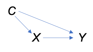
Figure 2.1: A confounding variable \(C\) on the effect of \(X\) on \(Y\).

For example, let’s say researchers investigate the effect of a master’s degree on adult earnings. They survey a large number of individuals and record whether they have a master’s degree and their earnings. Socioeconomic status is a confounding variable. Individuals with higher socioeconomic status are more likely to earn master’s degrees. In addition, they are more likely to have higher adult earnings, regardless of whether they have a master’s degree. For this example, let’s assume socioeconomic status is the only confounding variable. If the researchers observe an association between master’s degrees and earnings without information on socioeconomic status, it is not possible to determine if the association is due to an effect of master’s degrees or the effect of socioeconomic status.

2.4.2 Collider

Figure 2.2 depicts treatment \(X\) with no effect on outcome \(Y\). \(X\) and \(Y\) are both causes of collider \(Z\) (the two incoming arrows collide). The box around \(Z\) indicates conditioning upon \(Z\) in the analysis. In this case, there will be an association between \(X\) and \(Y\) even though there is no treatment effect. Figure 2.2 is a common way to depict selection bias where an association in subjects selected for the study is not present in the general population. In the selection bias diagram, \(Z\) is an indicator of selection into the study with a box around it because researchers only observe subjects selected into the study.

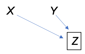
Figure 2.2: Collider \(Z\) with no treatment effect of \(X\) on \(Y\).

A very famous example appears in Pearl and Mackenzie (2018). In the general population, we would not expect to see an association between an individual’s talent and looks. More talented people are not better looking and vice versa. However, if we look only at famous Hollywood actors (\(Z\)), we would see a negative association between talent and looks in this group because an individual needs either talent or looks (or both) to become a famous Hollywood actor. Being less talented makes it more likely the actor is good looking because there must be some reason they became a famous Hollywood actor. More seriously, selection bias is a huge issue in medical and public health studies resulting in easily misinterpretated associations (Hernán, Hernández-Dı́az, and Robins 2004; Cole et al. 2010; Elwert and Winship 2014). For example, several studies have found a protective effect of smoking on Covid-19 infections (see Exercises).

2.4.3 Mediator

Figure 2.3 depicts mediator \(M\) of the effect of treatment \(X\) on outcome \(Y\). In this case, \(X\) is a cause of \(M\), \(M\) is a cause of \(Y\), and there is no effect of \(X\) on \(Y\) that cannot be explained by the effect of \(M\) on \(Y\). A common mistake is to adjust for \(M\). If we adjust for \(M\), we will not observe an association between \(X\) and \(Y\) when there is an effect of \(X\) on \(Y\).

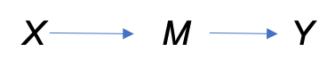
Figure 2.3: Mediator \(M\) of the effect of treament \(X\) on outcome \(Y\).

For example, let’s say researchers are investigating an adverse reaction to a medication using a treatment group and a control group where the adverse reactions are always preceded by increased blood pressure. Even if there is an effect of the medication on the adverse reaction, when we condition upon experiencing increased blood pressure, we will not observe an association between the medication and adverse reactions. Unfortunately, some researchers condition upon everything they measure, often resulting in poor estimates of effects (Hernán et al. 2002).

Exercises

1. You investigate the effect of a college education on adult earnings by surveying 1000 adults in your area and ask them if they have a bachelor’s degree (Y/N) and their yearly income in dollars. You find the college graduates earn about $30,000 more per year on average than the high school graduates.

1. Name the treatment and outcome variables in your study.

2. Is this an observational study or randomized controlled experiment? Explain.

3. Explain what it means for college education to cause higher adult earnings. In addition, explain how this differs from college education being associated with higher adult earnings.

4. Identify and explain a potential confounding variable in your study. (Be sure to explain how your confonding variable is a common cause of both the treatment and outcome).

5. Draw a causal diagram depicting the relationship between the treatment, outcome, and your confounding variable.

6. You also ask whether the individual has a Master’s degree (Y/N). What type of variable is having a Master’s degree? Redraw your diagram with this variable included in it.

2. Several studies have found a negative association between smoking and Covid-19 infection. Read “The spectre of Berkson’s paradox: Collider bias in Covid-19 research” and answer the following questions.

1. Explain what it means for smoking to cause a reduction in Covid-19 infections.

2. What type of variable is hospitalization in Figure 2?

3. Explain why many studies observe a negative association between smoking and Covid-19 infection.